Commonly used Algorithms
Machine Learning is used by different companies in multiple industries to solve their business challenges. The main reason for selecting Machine Learning algorithms over traditional algorithms is the accuracy in prediction they provide. Machine Learning helps in building a model which can produce a highly accurate model which further improves itself with an increase in training data.
Each of the four main types of Machine Learning can use a variety of algorithms. A summary of these main algorithms is provided below, along with some business use cases.
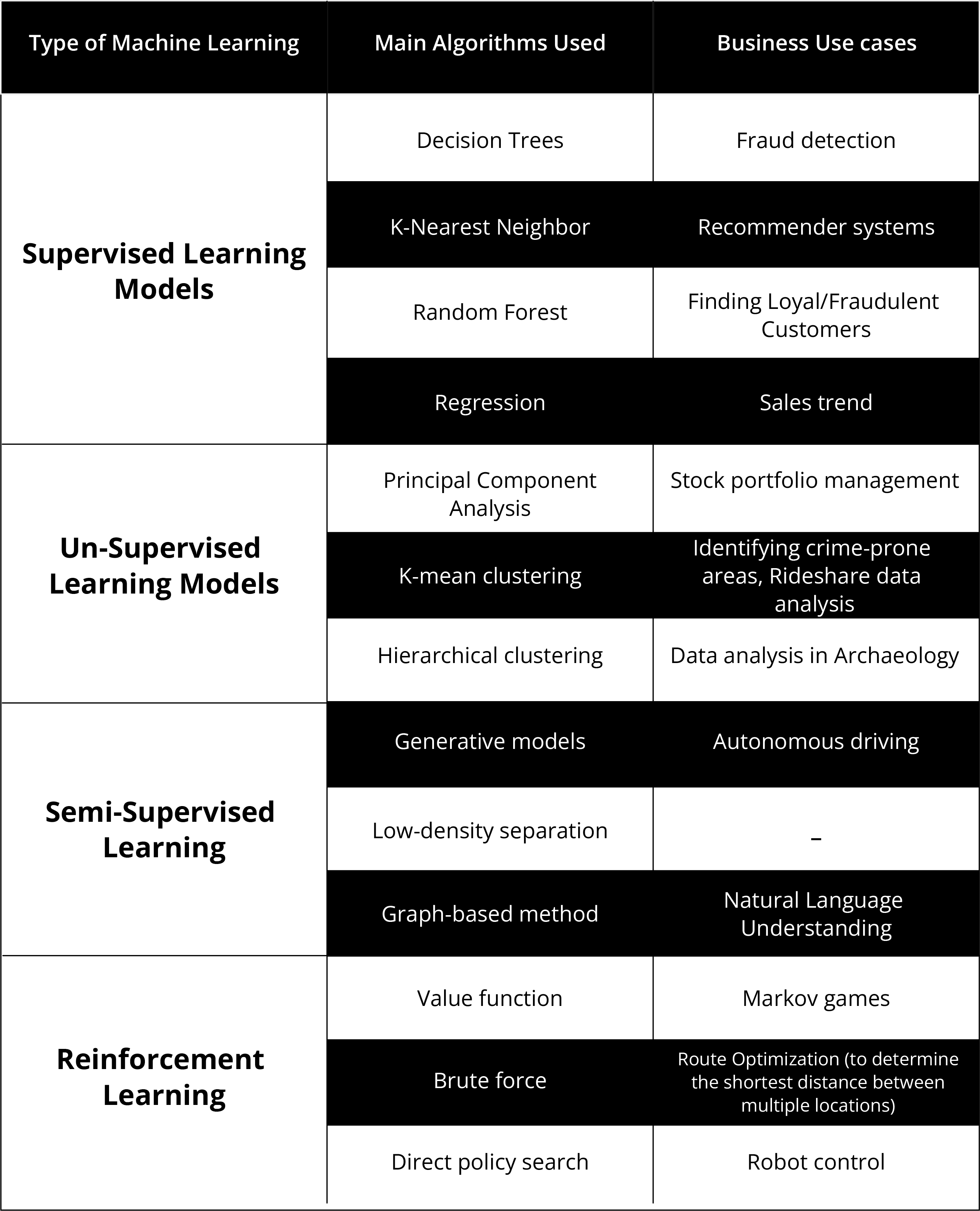 Main Machine Learning Algorithms and Some Key Business Use Cases
Supervised Learning Models
As we know Supervised learning models are used for labelled data and for regression and classification problems. A wide range of supervised learning algorithms are available, and each one comes with its inherent strengths and weaknesses.
Classification Algorithm
Classification is a technique where we assign the input data to a class or category. The prediction made by a Classification algorithm usually falls into a binary choice, for example: Is this email spam or not? Is this transaction fraudulent or not? Depending on the data and situation, there are different classification algorithms that could be appropriate:
- Decision Trees
- K-Nearest Neighbor
- Random Forest
Decision Trees
Decision Tree algorithms are insightful as with a small amount of data as they can show where the critical parts of a process lie. However, as the Decision Trees get more complicated, they can be inaccurate as a small change can lead to significant variances as you move downstream.
A decision tree is a flowchart-like structure in which each internal node represents a "test" on an attribute. Depending on whether the condition is met or not, the algorithm goes down a different path at each node. Each branch represents the outcome of the test, and each leaf node represents a class label. The paths from the root to the leaf represent classification rules. For multiple rules-based situations, these kinds of algorithms are the best.
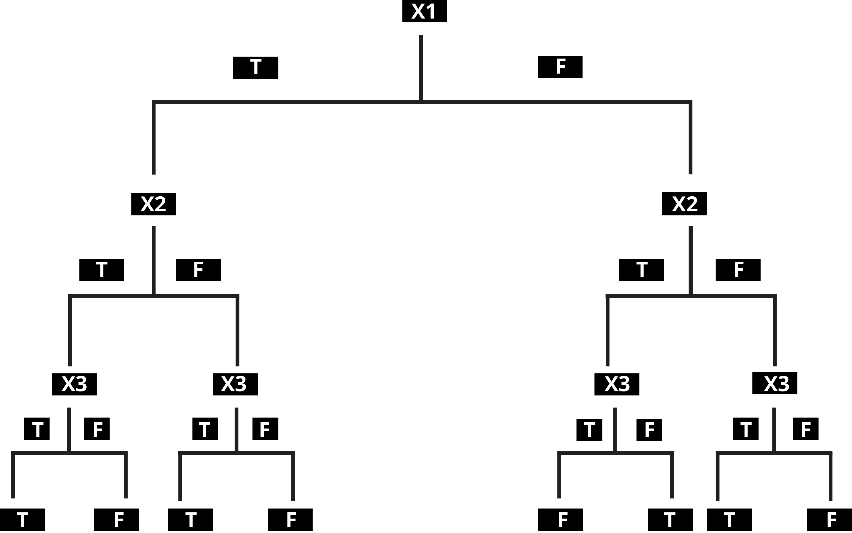 A Typical Decision Tree
Typical Use Cases
Decision Tree algorithms are especially useful when the goal of the exercise is to understand how critical each decision in the decision-making process is. A typical use case for these algorithms is fraud detection.
These algorithms are used quite often in understanding the types of transactions (e.g., chip or no chip, card present or not present, etc.), $ thresholds, the geography of the merchant, the geography of the user, the demographics of the user, and so on. Mapping out these variables can help bubble up commonalities in fraudulent transactions.
K Nearest Neighbor Algorithms (KNN)
We can use KNN for both classification and regression predictive problems. KNN is unique in that it is an algorithm that runs when executed. It does not store information or learn with time. It is typically run on small data sets.
KNN algorithms are used to find a predefined number of training data points closest in distance to the test data or new data and predict the label from training data. The number of observations can be constant K (user given) or based on the local density of points. KNeighborsClassifier and RadiusNeighborsClassifier are two types of algorithms that fall under the Nearest Neighbors Classification.
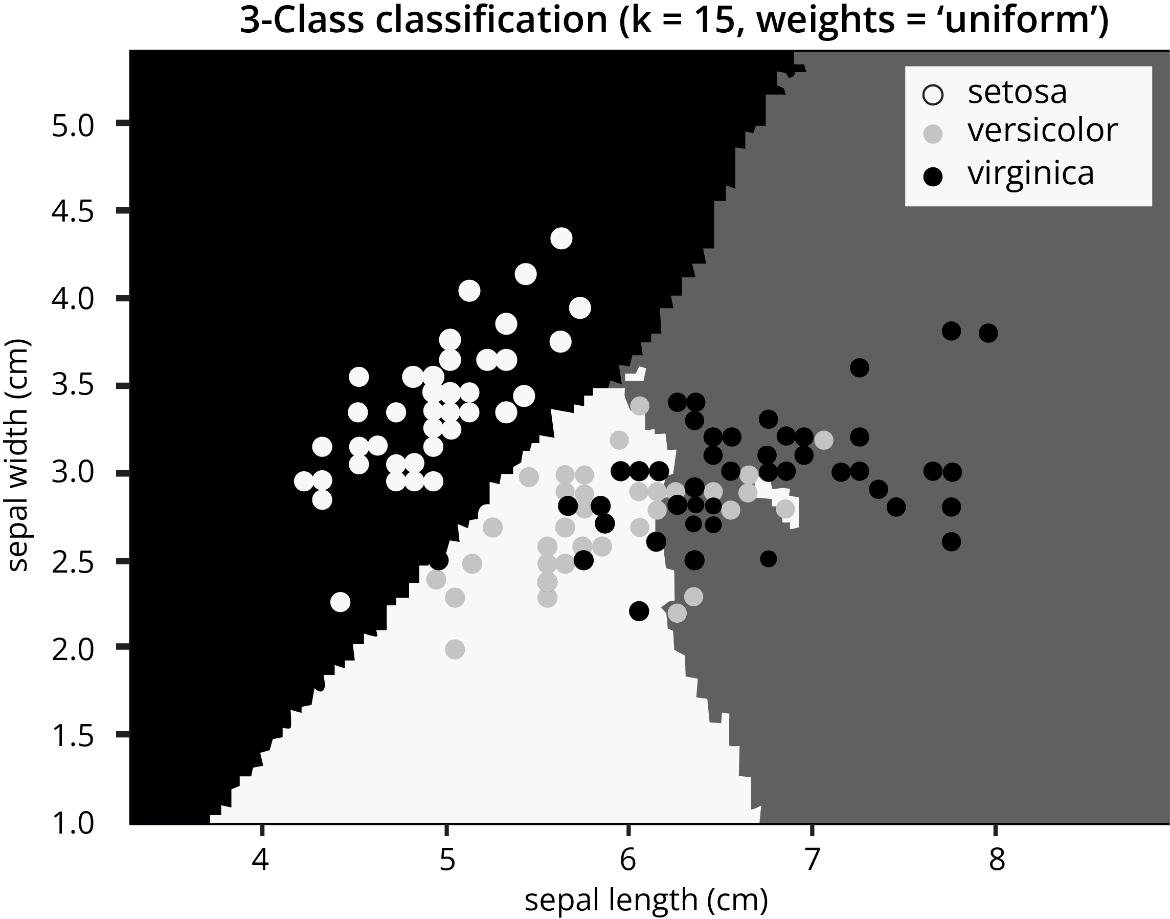
Simple recommendation systems, image recognition technology, and decision-making models often use KNN. It forms the foundation of companies like Netflix or Amazon when recommending different movies to watch or books to buy.
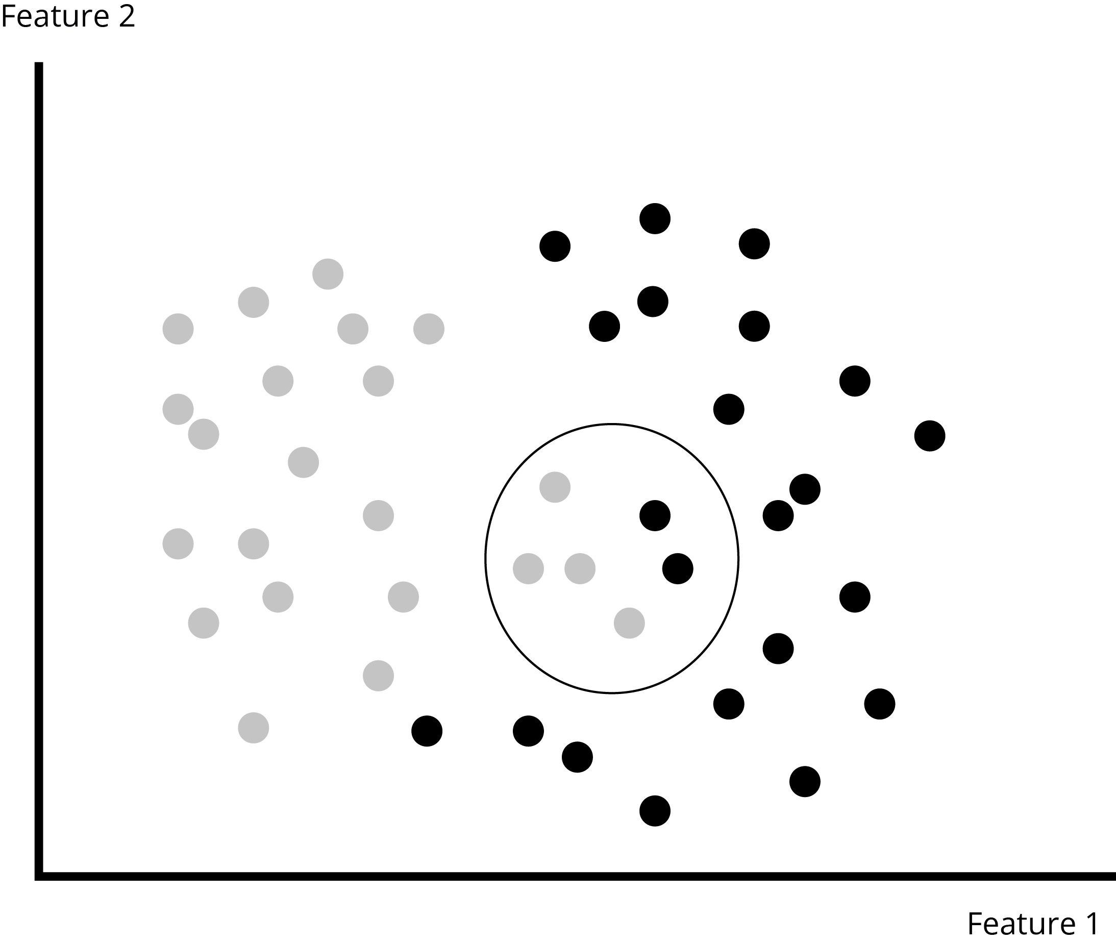 A Visual Representation of Cluster Analysis
Typical Use Cases
KNN powers simple recommendation systems to a large degree.
Based on available customer data and a comparison of other customer behaviour that is close to you, i.e., who have watched similar movies or bought similar books, it will give you a recommendation that will feel quite relevant.
Random Forest
Random Forest is another important algorithm that comes under the Ensemble learning algorithm category. In Ensemble learning algorithms, multiple models are built and the best-performing models amongst them are selected. Random Forest is a Bagging method of Ensemble Learning and GBM (Gradient Boosting Machine) is a Boosting algorithm of Ensemble Learning.
Random Forest builds multiple decision trees and merges them to get a more accurate and stable prediction. One significant advantage of Random Forest is that it can be used for both classification (grouping) and regression (checking for relationships) problems, which form the majority of current machine learning systems.
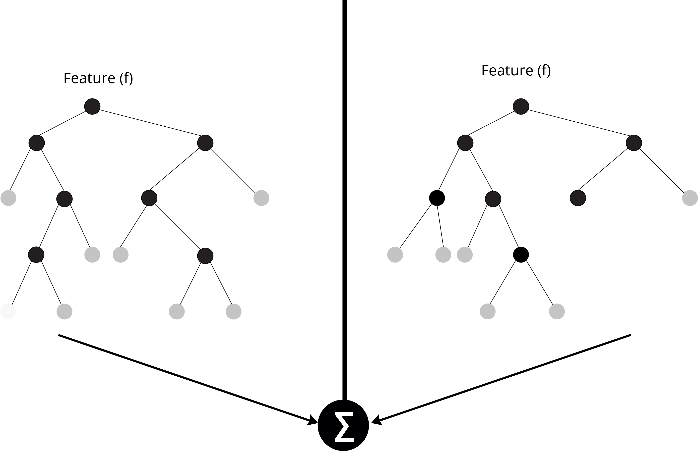 Merging of Decision Trees in the Random Forest Approach
Instead of searching for the most important feature while splitting a node, the Random Forest searches for the best feature among a random subset of features. This results in a wide diversity that generally results in a better model.
Typical Use Cases
An algorithm like Random Forest can help determine the preferences for future purchases of customers identified as loyal. A 2018 study in the Middle East shared its results publicly and called out Random Forest models as one of the two approaches that displayed accuracy of between 93–96% for customer retention on a telecom customer dataset.
Regression
Regression is a technique which tries to predict a continuous value for the input based on the available information. The most simple model used here is the Linear Regression model. This model has been the most widely used statistical technique in business and economics.
For example, if a company had a successful sales season repeatedly for the holiday season for a few years, it can use linear regression to predict future sales for the upcoming holiday season. Similarly, the company can use it to forecast the pricing and promotions of a product.
Assumptions in Linear Regression
This model has limited capability in some situations. The key assumptions that this model makes are as follows:
Linear regression works best when the relationship between the independent and dependent variables is linear. It assumes a straight line can be plotted when it comes to the different values of the input variable to the output variable.
Input variables should be independent of each other, this means there is no relationship between Input variables.
Linear regression is sensitive to outliers. But in the real world, the data is often contaminated, and outliers should be adjusted. This is easier said than done as it is hard to differentiate between what is noise and what is a real observation.
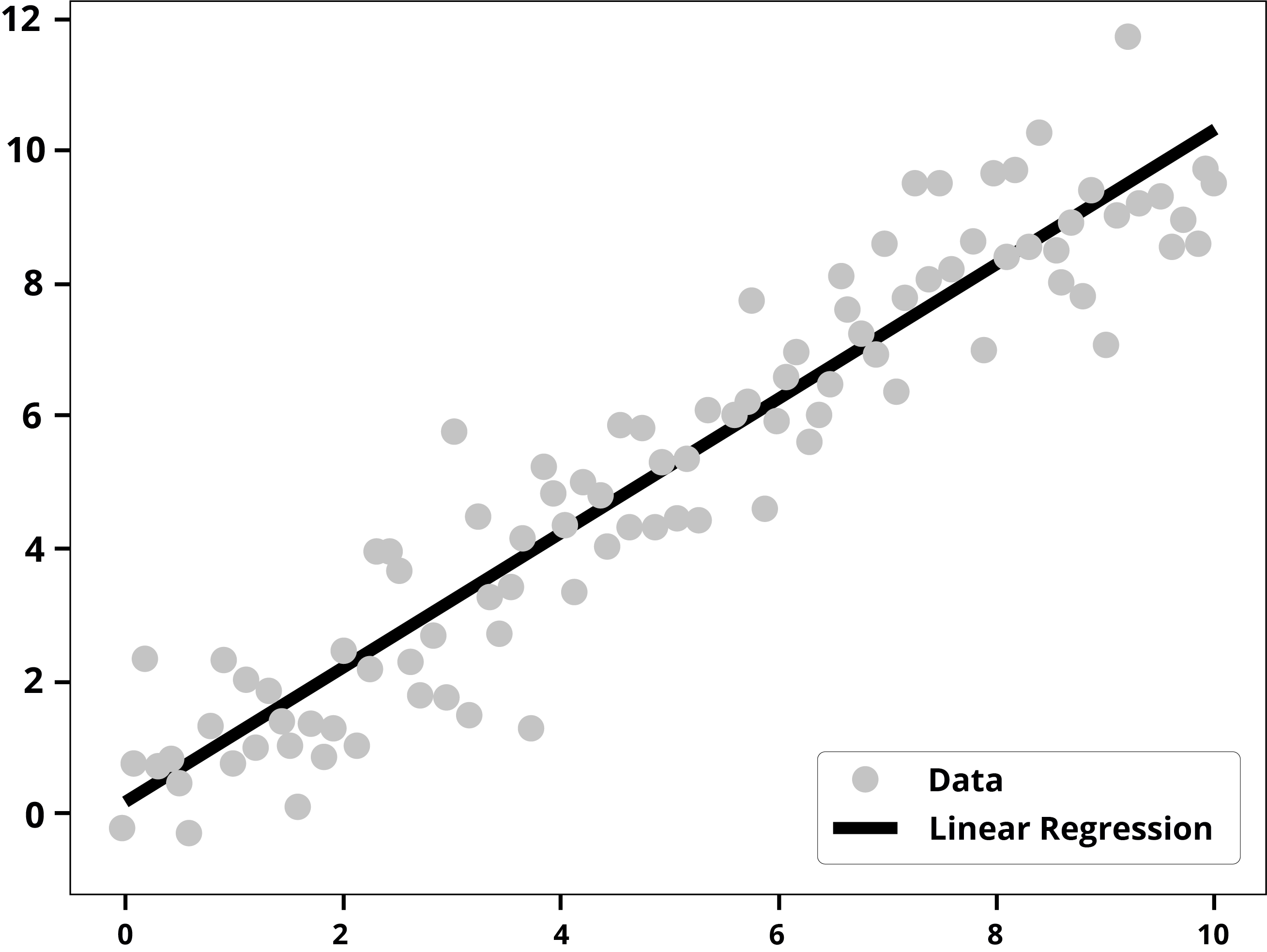 Visual Representation of a Linear Regression
Typical Use Cases
Linear Regression is the most useful and frequently used algorithm. We can use linear regression for sales forecasts which can help businesses in planning and budgeting. Sales can be predicted using marketing expense, customer footfall and other variables.
Sales = 0+1*MarketingExpense+2*CustomerFootfall
There are many use cases where we can use linear regression like sales forecasting, stock price prediction, predicting customer behavior and many more.
We use Linear regression to evaluate trends in business and make better future decisions. The trend line created uses a ‘best fit’ approach where the model tries and achieves the best possible outcome with the least amount of inaccuracies.
Unsupervised Learning Models
Unsupervised Learning Models are used for unlabeled data to identify similarities and patterns in different data points. The data points which show similar patterns are grouped together and are called a cluster. These clusters can be analyzed by the marketing team to offer different products and different offers to different clusters.
Let us examine the central Unsupervised Learning Models and the standard techniques that are mostly used.
Clustering
Clustering is used mostly for unsupervised learning models and algorithms. But in some special cases we use clustering in supervised learning models as well. Supervised clustering is used for image segmentation, news articles clustering and streaming email batch clustering. Here the algorithm is used to learn from training data to parameterized item-pair.
Clustering is the task of grouping sets of similar objects together. Cluster analysis itself is not one specific algorithm. Clustering can be achieved by various algorithms that differ significantly in their understanding of what constitutes a cluster and how to find them efficiently.
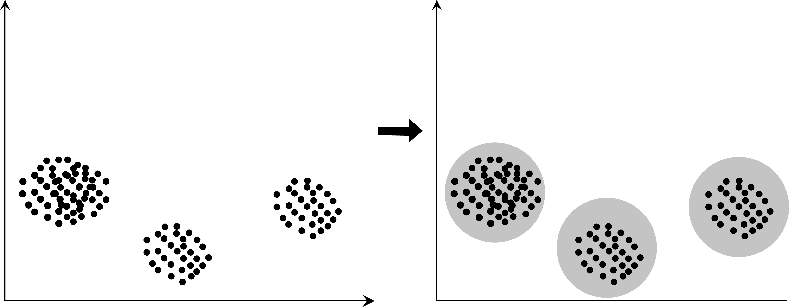 A Visual Representation of Clustering
Typical Use Cases
Clustering is widely used when it comes to grouping customers and segmenting buyers by dividing the customers into segments and grouping them by their shopping behavior. Businesses can use this approach with other analytical tools to manage their data better.
The two most widely used techniques for clustering are:
- K-mean clustering
- Hierarchical clustering
In K-means clustering the data is partitioned into clusters based on their means. Thus the closer the data points to each other, the more similar they are taken to be.
Hierarchical clustering follows a similar approach to K-means but takes the results one step further. Hierarchical clustering treats each data point as a cluster and merges the closest data points with each other until a few key clusters remain. The output of this approach depends on the minimum distance between each cluster that can be specified and the point where this minimum distance should be applied.
Principal Component Analysis
Even though we have made significant advances in computing power and storage costs, it still becomes difficult to process data with higher dimensions. So dimension reduction methods tend to squeeze data size only to relevant features and neglect the rest as noise. One of the techniques that help through this process is PCA (Principal Component Analysis).
We try to find a set of relevant variables and combine them into a single collection consisting of essential variables. These new sets of variables are called principal components, which should be fed as inputs to the learning model.
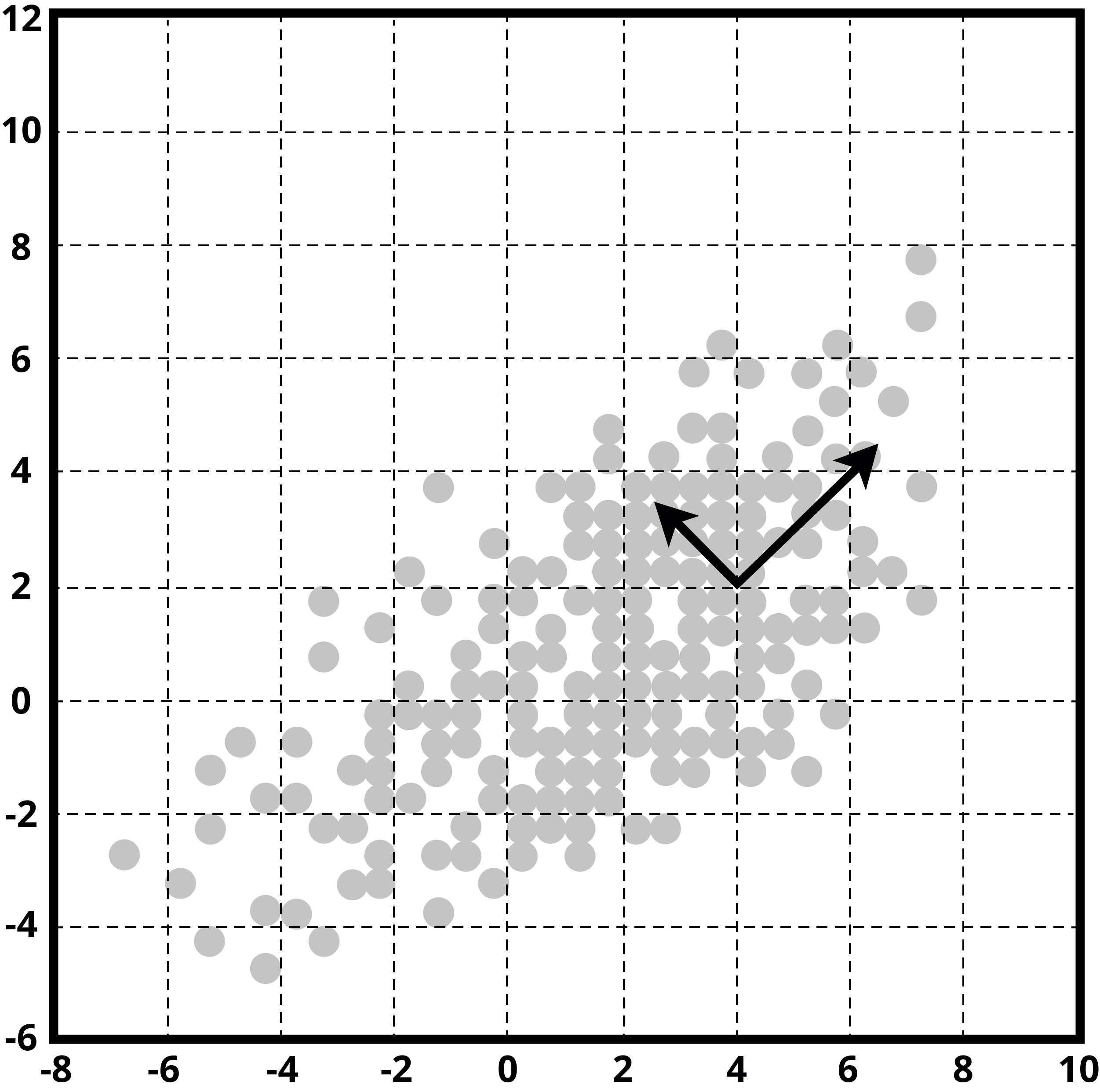 Determining Principal Components
Typical Use Cases
Let's say we have to analyze 1,500 stocks in a portfolio. Let's further assume that we have a hundred key variables for each stock. This assumption would give us 1,500 X 100 = 150,000 variables or combinations to be examined, sorted, and scored.
It is going to be a burdensome task, even with high computing power. Upon examining the data we may find that as our goal may be to judge 30-day stock price performance, data points like intra-day high and intra-day low are data points that add no value and do not impact the model accuracy. By identifying such variables, we begin to remove the data points that do not add any value to the problem statement that was formulated.
A key takeaway of the PCA approach is that as a user we can create a hybrid variable too if we think that it will assist in the accuracy of the model prediction.
Semi-supervised Learning Models
We will examine three main semi-supervised learning models that we commonly use.
- Generative models
- Low-density separation
- Graph-based methods
Generative Adversarial Networks (GANs)
Semi-supervised learning based on generative adversarial networks (GAN) have been used in the application of autonomous car driving. GAN models effectively capture the data distribution and hence create a powerful representation of the data. This gives us the ability to generate a realistic dataset for the framework of autonomous driving.
Under the GAN approach two models are engaged in competing with each other (hence the use of the word ‘adversarial”) resulting in better accuracy over time. The first GAN is the ‘generator’. This generator comes up with new likely examples e.g. if the goal is to detect cancer cells, the generator will come with new images of what cancerous cells may look like.
The other GAN, the ‘discriminator’ learns to classify the artificial examples from real examples. And over time the discriminator becomes better and better as it makes its way through more data.
Typical Use Cases
GANs have found a lot of use in facial image recognition, image classification, face ageing and the creation of personalized emojis out of images. Understanding how GANs work, will hopefully assist you in understanding why that is the case.
A 2019 study shows that graph-based methods in semi-supervised learning have reduced the error rate of the NLU (Natural Language Understanding) model by 5%. This technology is crucial for voice assistants like Amazon’s Alexa, Google’s Home, and Apple’s Siri.
Low-Density Separation
The Low-Density Separation approach is related to Cluster Analysis. An outcome of the Cluster Analysis is an area of the high-density region. If two data points are close, that means they belong to the same cluster or their label must be the same. Low-Density Separation is used to separate data points using low-density regions. The samples belonging to low-density space are mostly likely to be boundary points or their classes can be different.
We know the Supervised algorithm SVM (Support Vector Machine), where the support vector lies in a low-density region. Low-Density Separation methods attempt to find decision boundaries that best separate one label class from the other and identify a label for unlabelled data points. The Transductive Support Vector Machine (TSVM) is an example of Low-Density Separation.
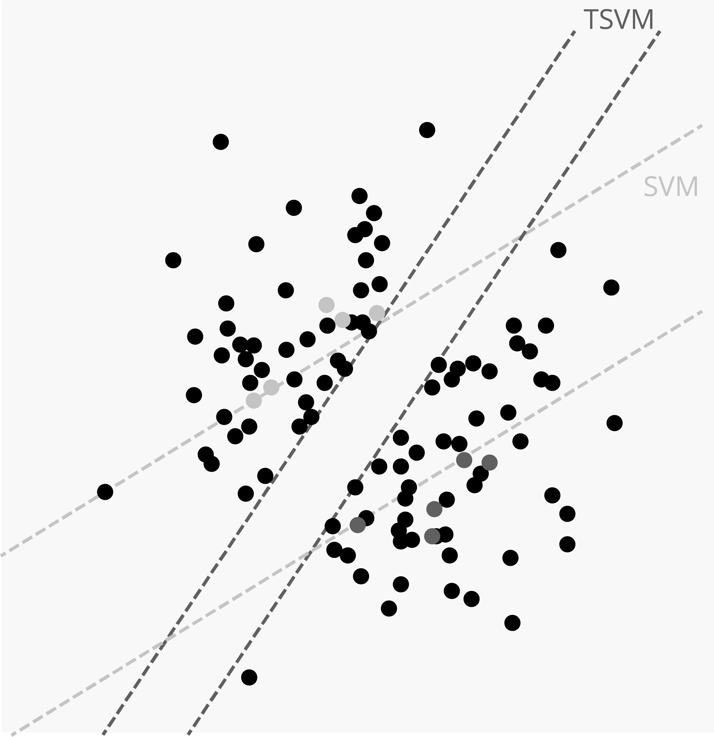
Typical Use Cases
Low-density separation - Handwritten Digit Recognition.
The Low-Density Separation method uses many real-world problems such as text classification. It can be used for handwritten “Digit Recognition”. For example, we may want to distinguish between the handwritten digit “0” against digit “1”. A sample point taken exactly from a decision boundary will be between “0” and a “1”, will help in such a determination .
Low-density separation will be trained on large datasets which include some labelled data and large amounts of data as unlabelled. It will learn the pattern of writing digits from labelled data and apply it for unlabelled data.
Graph Based Methods
A graph, in Machine Learning, is a data type that has nodes and edges. And, both nodes and edges can hold information.
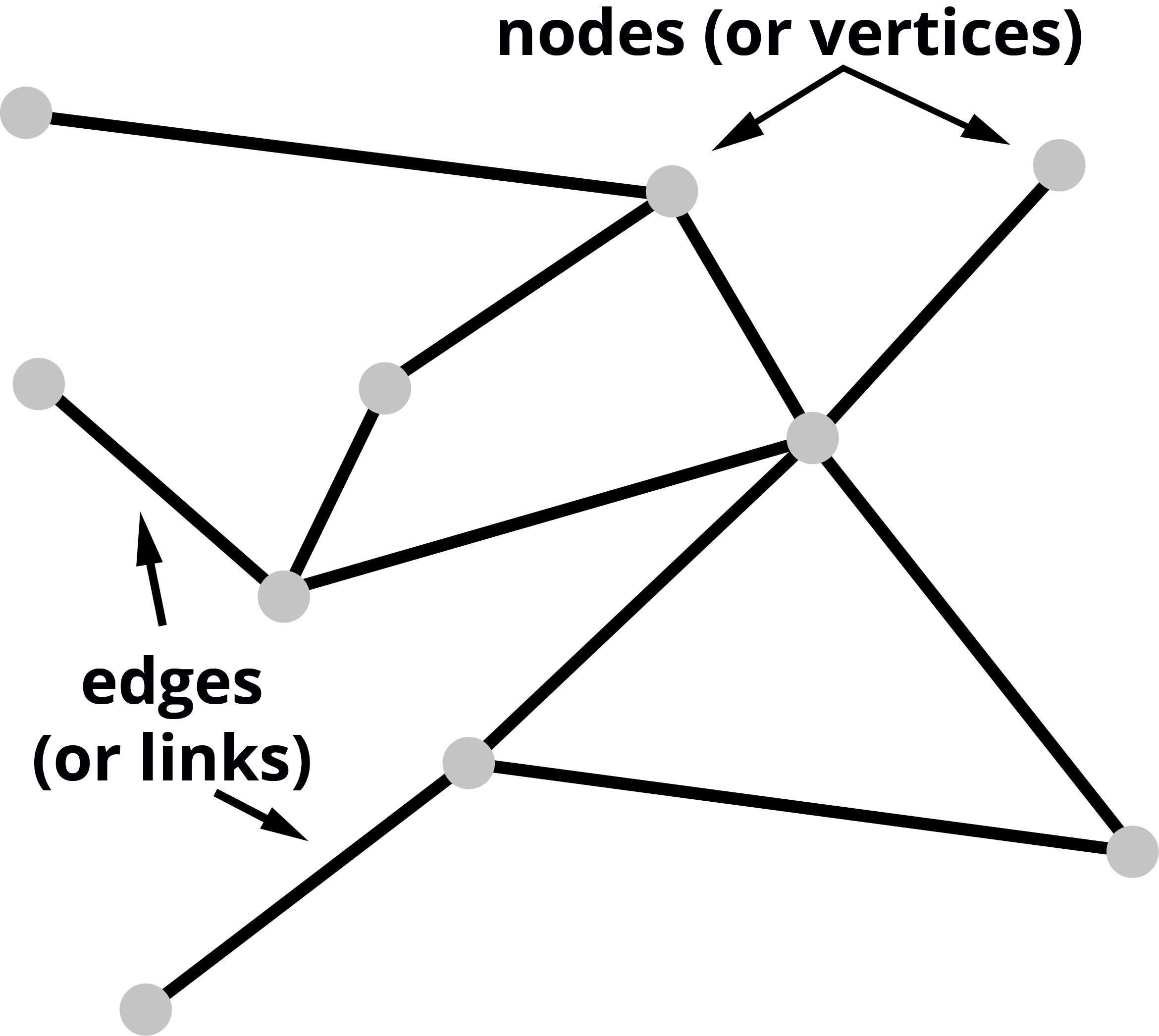
Edges can represent direction indicating the flow of information and the nodes can be representative of weights.
According to Widmann and Verbern, Graph-Based Semi-supervised Learning (GSSL algorithm) is very effective for different kinds of problems specifically for short text classification. The GSSL algorithm uses either graph to spread labelled labels data to unlabeled data or to optimize the loss function. In the graph-based method, we build a complete graph-based model on similarities between the label and unlabeled nodes. The nodes which have high similarity trends have the same label.
The advantage of the GSSL algorithm is that it converges quickly and can be easily scaled for large data. It is also flexible to adopt but its computation is complex and expensive.
Typical Use Cases
The graph based approach is easy to imagine when we think of social networks like Facebook. The re-prioritization of the items in the news feed that was first announced in 2018 was a reflection of the graph theory that has been continuously built upon.
By prioritizing personal messaging over brand messaging and within that, prioritizing posts that indicate or lead to a more meaningful conversation or were from a closer circle of friends, were indicative of the graph-based approach at work.
Reinforcement Learning
Reinforcement learning, due to its generality, is studied in many other disciplines, such as game theory and simulation-based optimization. A key concept in Reinforcement learning is the concept of rewarding a machine and hence being able to bias its behaviour to complete tasks sooner or more efficiently.
A reinforcement learning agent interacts with its environment in discrete time steps. At each step, the agent receives a reward. The agent then chooses an action from the set of available actions. With reward maximization as its goal, the algorithm can work out how best to complete a given task.
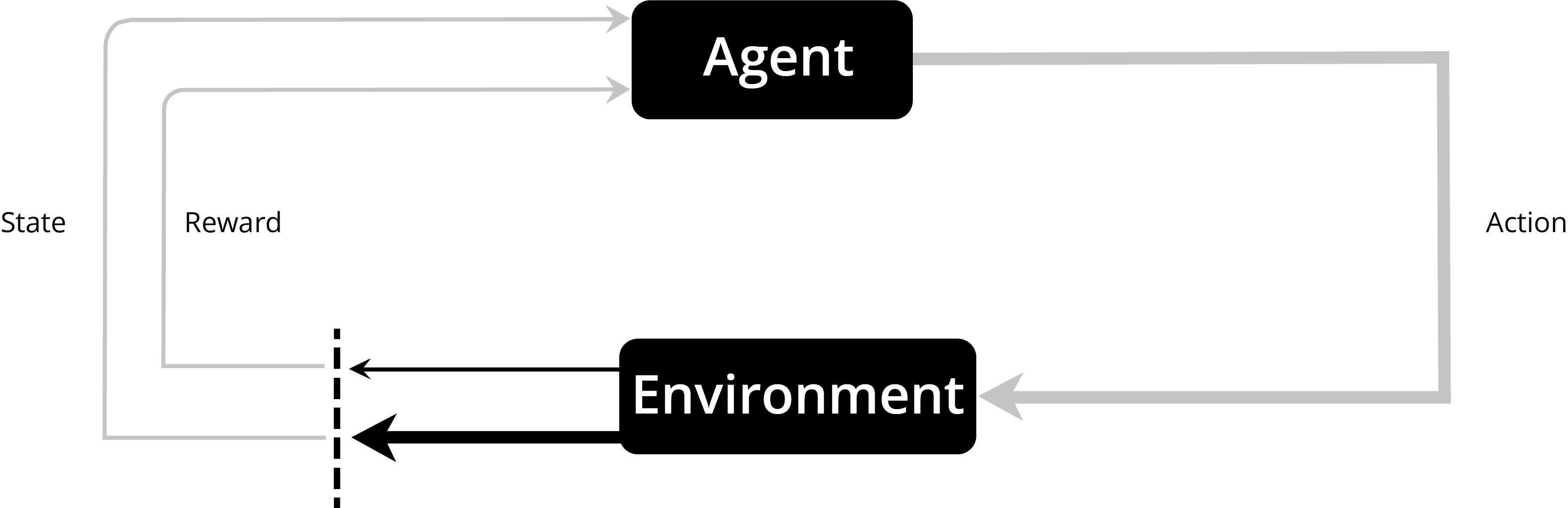 A Visual Representation of Reinforcement Learning
Let us examine the main reinforcement learning models.
- Value function
- Brute force
- Direct policy search
Value Function (Q-learning)
Q-learning is a technique that tends to find the best action in a given environment. This algorithm updates the value function and seeks to maximize the total reward.
Brute Force
Brute Force-based learning attempts to take into account all possible options into account. When the problem is manageable, the need for computing resources is acceptable and the options are limited or when the cost of a mistake is high, this may be an option that can be considered.
Typical Use Case
Consider a Level 5 self-driving car, where there is no plan to have a steering wheel, gas pedal, brake, etc. and the machine is supposed to take care of everything. The human passenger cannot take any evasive action in case of an emergency. Due to the high-cost litigation in the case of an accident, a Brute Force approach may be the best way to try and solve this problem.
Clearly, this approach should only be used in a select few situations.
Direct Policy Search
The Direct Policy Search approach utilizes options (policies) where the agent (program) seeks to maximize its reward. The policy can differ with differing environments. The agent here takes a completely different approach than in the case of Brute Force.
The agent can be fed different policies or the agent can learn and devise its own policies over time.
Agents can use the Markov strategy where they have a history of having tried out a few different options in memory and are aware of the overall reward at stake. In such situations, the agent calculates the next moves based on the overall objective. It does not use a brute force approach and does not use a programmed Direct Policy approach, but can come up with newer policies too.
Typical Use Cases
Typical use cases of the Direct Policy approach can be found in building a Robot Control system. Policy search methods have made tremendous development like learning trajectory-based policies for complex skills and learning complex policies with thousands of parameters. But building Robot-RL is still challenging.
Direct Policy search is also used for tracking autonomous underwater cables by visual feedback, autonomous helicopter control, and learning obstacles avoidance parameters from operator behaviour.
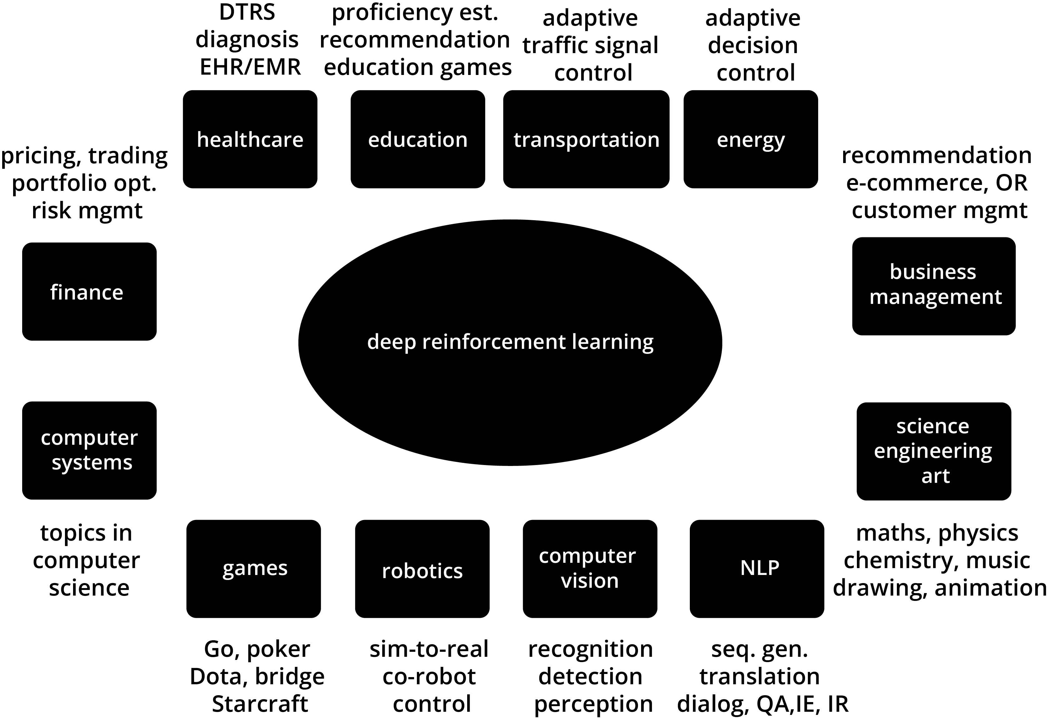
From recent advancements in technologies and research, there are many use cases of reinforcement learning. You can see some of it in the below image as well.